LiCSAR proc

This section describes core functionality of LiCSAR system, that is used by LiCSAR FrameBatch system but can be used independently. Some parameters of particular use (often not fully integrated in FrameBatch) are discussed here, yet we assume that you work with standard project started by licsar_make_frame.sh. Some more information can be found in LiCSAR Wiki and materials from COMET InSAR workshops.

In principle, LiCSAR_proc codes are built on top of GAMMA software for the main processing (as set of wrappers, enhanced by functions we developed or imported from existing open-source projects, such as GMT, GDAL, Doris and a bunch of python libraries).

Forming LiCSAR interferograms (Sentinel-1)

The core processing scripts are also described (in more details, and still valid, although of older date) in CIW 2019 LiCSAR Tutorial.

1. create SLC files

see

LiCSAR_01_mk_images.py -h

normal use:

frameid= # e.g. 016A_02562_091313
m= # reference date, e.g. 20191103
s= # e.g. 20220101
e= # e.g. 20220201
LiCSAR_01_mk_images.py -n -d . -f $frameid -m $m -s $s -e $e -a 4 -r 20

This command would create SLC for given frame in given time period. For this to work, you should be sure the data are existing on disk and are ingested to LiCSInfo database (command arch2DB.py). This is done automatically through licsar_make_frame.sh.

To have it run without frame definitions, see CIW 2019 LiCSAR Tutorial and explore -y,``-p`` and -l parameters.

2. coregister to RSLC files

see:

LiCSAR_02_coreg.py -h

normal use:

frameid= # e.g. 016A_02562_091313
m= # reference date, e.g. 20191103
LiCSAR_02_coreg.py -f $frameid -d . -m $m -i

This command would coregister/resample all files in SLC folder to RSLC directory, for given frame. Explore other parameters (see -h) on how to list epochs to process etc. Note that by default, the script would regenerate geo files based on DEM and the primary epoch metadata - this can (and often should) be skipped by -i parameter. The standard constrains apply, for example limit for spectral diversity estimation to combine epochs with up to Btemp=180 days.

Note:

In order to force-skip the 180 days limit, use parameter ‘-E’ (some extra tweaks there, EIDP-related, including skip of Btemp check). In practice, to connect a cluster of epochs far in time, choose one SLC in that cluster that has no missing bursts (see e.g. their mli preview, or check size), and add its date to slclist.txt and try coregister that one by LiCSAR_02_coreg.py -f $frameid -d . -m $m -i -l slclist.txt -E. Only then start the standard procedure (without -E) for all the SLCs left. This way you would make sure that the other epochs would use appropriate RSLC3 for the spectral diversity (see e.g. https://www.mdpi.com/2072-4292/12/15/2430 ). This approach would be automatically run through the LiCSAR FrameBatch script with ‘force’ parameter: framebatch_postproc_coreg.sh -f.

3. create interferograms

see:

LiCSAR_03_mk_ifgs.py -h

The script is very useful if you have your own list of interferograms to form, e.g. in a text file containing lines as ‘20200101_20200202’ etc. (see help). An extra parameter -n would use parallel processing on given number of CPUs.

The interferograms are generated by default with 20/4 multilooking factors in range/azimuth. Then, the coherence is calculated (using GAMMA’s cc_wave) as a result of 5x5 window convolution. The interferometric phase is then filtered (using GAMMA’s adf). The default filter parameters are: alpha=1, window size=32x32 (see global_config.py for default parameters). Finally, the interferograms (and coherence) are geocoded to WGS-84 in 0.001 degrees resolution, by default.

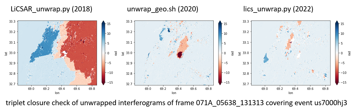
4. unwrap interferograms

For the original unwrapping approach, running on radar-coordinate interferograms, use:

LiCSAR_04_unwrap.py -h

and then you may geocode the result, as discussed in next section. By default, it would mask pixels with coherence lower than 0.35.

However, you may find useful (and faster) the updated version, currently used by LiCSAR FrameBatch, that performs unwrapping on already geocoded wrapped interferograms:

unwrap_geo.sh

In this case, the masking is done only with landmask (GMT feature) and only points of coherence below 0.05 are masked.

Finally, you may experiment with the updated (much improved) unwrapper, running through python, and starting again from geocoded interferograms. This script is used by licsar2licbas.sh described later.

import lics_unwrap as unw
help(unw.process_frame)
help(unw.process_ifg)

To provide a general overview of differences between those three options (using default parameters), see the image below (as presented at IGARSS 2022 ). Basically, unwrap_geo.sh would underestimate strong deformation but would not be that prone to general unwrapping errors. The third option is result of active development (and will further improve). So far the best option.

General comparison of the three unwrapping approaches by the triplet closure test

5. geocoding results

For geocoding results, please use the following command:

create_geoctiffs_to_pub.sh

Post-processing

Reunwrapping existing interferograms

Standard LiCSAR products use general parameters for unwrapping. Here we document the python tool lics_unwrap.py that performs published procedures . This approach is implemented in LiCSBAS as LiCSBAS02to05_unwrap.py and details available at API documentation.

To show an example, this is how we could use range offsets [px] to support unwrapping:

from lics_unwrap import *
ifgdir = '/gws/nopw/j04/nceo_geohazards_vol1/public/LiCSAR_products/21/021D_05266_252525/interferograms/20230129_20230210'
phatif = os.path.join(ifgdir, '20230129_20230210.geo.diff_pha.tif')
cohtif = os.path.join(ifgdir, '20230129_20230210.geo.cc.tif')
rngtif = os.path.join(ifgdir, '20230129_20230210.geo.rng.tif')
ifg=load_from_tifs(phatif, cohtif)
prev_estimate=load_rngoffsets_as_prevest(rngtif, thres_m = 9, golditer = 3)
ml10 = process_ifg_core(ifg, ml=10, tmpdir = 'test', fillby = 'nearest', goldstein = False, smooth = False,
                        lowpass = False, defomax = 1.2, gacoscorr = False, pre_detrend = False,
                        prevest = prev_estimate)
ml10.unw.plot(); plt.show()

LiCSAR to LiCSBAS (JASMIN)

This script runs LiCSBAS processing from the LiCSAR data. To be used in JASMIN environment.

The script would read frame data from $LiCSAR_public directory, prepare them for LiCSBAS and run LiCSBAS with default parameters. If you run the script from directory with your GEOC outputs, it would instead use the local data from this folder. Afterwards, you may just fine tune parameters of LiCSBAS step 15 (and 16) and rerun them, for the final result.

licsar2licsbas.sh frame [startdate] [enddate]
#e.g. 155D_02611_050400 20141001 20200205
#Parameters:
### Basic parameters
##-M 10 .... this will do extra multilooking (in this example, 10x multilooking)
##-g ....... use GACOS if available for at least half of the epochs (and use only ifgs with both epochs having GACOS correction, other will be skipped)
##-G lon1/lon2/lat1/lat2  .... clip to this AOI
##-u ....... use the reunwrapping procedure
### Control over reunwrapping
##-c ....... if the reunwrapping is to be performed, use cascade (might be better, especially when with shores)
##-l ....... if the reunwrapping is to be performed, would do lowpass filter (should be safe unless in tricky areas as islands; good to use by default)
##-m ....... with reunwrapping with Goldstein filter on (by defaule), use coh based on spectral magnitude (otherwise nyquist-limited phase difference coherence) - recommended param
##-s ....... if the reunwrapping is to be performed, use Gaussian smooth filtering (this will turn off Goldstein filter, and disable -m)
##-m ....... use GAMMA ADF for filtering if Goldstein filter is selected (does not work together with -s)
##-t 0.35 .. change coherence threshold to 0.35 (default) during reunwrapping (-u)
##-H ....... this will use hgt to support unwrapping (only if using reunwrapping)
### Control over LiCSBAS processing
##-T ....... use testing version of LiCSBAS
##-d ....... use the dev parameters for the testing version of LiCSBAS (currently: this will use --nopngs and --nullify, in future, this will also add --singular)
##-W ....... use WLS for the inversion (coherence-based)
### Processing tweaks
##-P ....... prioritise, i.e. use comet queue instead of short-serial
##-n 1 ..... number of processors (by default: 1, used also for reunwrapping)

Explaining on example, use of

licsar2licsbas.sh -c -M 5 -u -T -g -s -W -G 5.1/5.2/3.3/3.5 100D_00000_010101 20150101 20160101

would grab wrapped interferograms of this (fictive) frame 100D that cover period of year 2015, then it will check for availability of GACOS corrections (-g) and use them if they exist for most of epochs (if you used -S, GACOS corrections would be applied only if they exist for ALL epochs). Then it would crop them to the coordinates given by -G, and then it will reunwrap them (-u) with 5x multilooking (so the resolution if using default LiCSAR data would become approx. 500 m), with support of cascade approach (-c) that means a longer wave signal is first estimated/unwrapped (using 10x the -M factor) and used to bind the final unwrapped result - therefore especially decorrelated areas would not induce unwrapping error.. hopefully. The cascade approach should give comparable results to use of the (simpler) lowpass filter (parameter -l) that we actually recommend to be used by default. Since the -s parameter was used, the interferograms are smoothed by Gaussian window instead of default Goldstein filter. No worries about spatial filtering - the residuals from the filtering are unwrapped and added to the result as well.

The data here will be prepared to folder GEOCml5GACOSclip. Then, the -T would use up-to-date LiCSBAS codes with their experimental functionality ON (in this case, e.g. nullification of pixels in unwrapped pairs with loop closure errors over pi is ON). Thus basically parameter -T would equal to LiCSBAS12 --nullify; LiCSBAS13 --nopngs, plus some fine-tuned parameters. In near future, the -T would also add –singular to the step LiCSBAS13. With the -W parameter, LiCSBAS13 performs weighted least squares for inversion where weights are estimated from coherence in each temporal sample of each pixel - this is more reliable.

The whole procedure will run in the background through JASMIN’s LOTUS server (see generated .sh files) and once finished, results will be in TS_GEOCml5GACOSclip, plus additional files will be generated (e.g. geotiffs of velocity estimate, or standard NetCDF file that can be loaded to e.g. QGIS or ncview to plot time series from ‘cum’ layer, etc.)

Finally, note the biggest impact in the unwrapping here is the spatial filtering approach. While the Gaussian smooth should run very well, some high phase gradient areas would benefit from Goldstein filter. Therefore this filter is ON by default (it would be turned off with -s) but it is recommended to add parameter -m and fine tune -t. The negative aspect of this implementation is the longer processing time, and also the method to measure noise is still in development.

Decomposition to E-U(+N) vectors

This section should contain information on both decomposition from A+D - for now, you may go through tutorial by Andrew Watson. For LiCSAR, you may investigate script decomposition.py for a simple solution in python (Andrew adds weighting average etc in his open MATLAB scripts).

Tools operating with LiCSAR data

LiCSAR Data Quality Checker

This tool is a GUI (fast-)programmed to fast-look into preview PNGs of LiCSAR interferograms, and fast-flag errors in them. Once the operator (you) flags erroneous data within selected LiCSAR frame, the software will auto-generates a small .savedResults file. If you inform us about bad interferograms in LiCSAR system by sending the file to our team, you directly help improve our open dataset, as we will remove and reprocessed the corrupt data. Additionally, if you are a student of University of Leeds, and you will run (after setting the environment as described here) lics_checker.py at some Leeds server, all your flagged data and the output .savedResults file will be stored in folder /nfs/a1/insar/lics_check, and thus we will be able to apply machine learning, once we prepare a long-wished workflow to auto-detect such errors.

The use of the tool is simple:

Run lics_checker.py (you may also download it from here, just make sure you install required python libraries if you run it from non-leeds-uni computer - just see the import lines in the script).
The tool will download list of LiCSAR frames. Select track and frame you want to look into. If this frame was already checked, it will not appear in the list, until you untick exclude checked.
Once you click OK, the tool will download existing png previews of wrapped and unwrapped interferograms - the output is shown in the terminal (together with info on output directory). Note, we actually notice some connection issues causing download to stuck - if this happens, just press CTRL+C, the program will continue downloading other pairs.
Once downloaded, you will see main screen of the viewer:

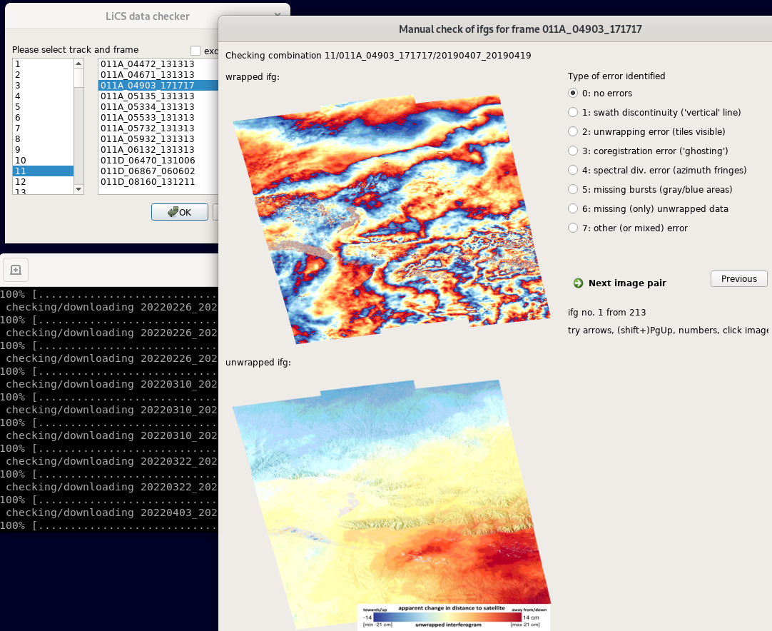
Here, you can flag type of error that you see - either by clicking on its radio button by mouse (by default: set to no error), or pressing key corresponding to the error’s number on your keyboard. To switch to the next image, either click on the ‘Next image’ button, or just press Right arrow. Especially using arrows, you can fast-scroll through the interferograms. You can also use buttons PgDwn, PgUp to scroll by 10 interferograms, or shift-PgDwn, shift-PgUp to scroll by 100. After the last interferogram, the program will notify you that it saved the results to a file (see terminal). Also, the results are auto-saved during the process, so your next check will use existing flags. To add, clicking on the preview you will see it in larger resolution.

And that’s all folks, happy flagging!